Outline Link to heading
Introduction Link to heading
Dataframes, data structures that are very similar to tables, are key elements in data science. They are extremely useful for organizing information, and many instances of data science use dataframes to clean and organize data, manipulate tabular data, and even to produce visualizations. The following tutorial aims to provide a basic overview of useful functions when working with dataframes.
It is completely normal to be googling functions and their usage, no matter what fluency you have in coding! There are so many methods towards the same solutions, so it is good practice to continously learn about all the coding possibilities, and then determining which ones you like best. I write this tutorial in hopes that I can compile some of the most common practices in one page and aid you in improving your coding efficiency! I will also link useful webpages if you are interested in learning more about any of the topics covered.
Notice Before following this tutorial, make sure you have Python and a source code editor (such as VSCode or Atom) installed. If you do not have Python, you can look here for installation instructions.
Reading a Dataframe Link to heading
Let’s start our code by importing important libraries. Libraries contain prewritten code that serve as tools for tasks that coders often have to reuse. The one that we need to import will be pandas.
import pandas as pd
Now, let’s create a dataframe. There are many ways to create a dataframe, as shown by the link above. However, arguably, many dataframes that you will be working with in class or in a job will be imported (usually as a .csv file); this is because dataframes are meant for working with large amounts of data, and coding a dataframe from scratch would be too tedious.
For this tutorial, I have created a downloadedable dataframe for you to practice with! However, feel free to practice coding a simple dataframe if you want to try!
To open up the csv file as a dataframe in your source code editor, type:
# df is the variable we are assigning the dataframe to in this example
# File path tells your computer where the csv is stored.
df = pd.read_csv("FIlE PATH TO CSV")

# An example of how the filepath may look like
df = pd.read_csv("/Users/daniellelouie/Documents/minecraft_wood_.csv")

# Print out the a view of the dataframe
df
Make sure you change the filepath to wherever you stored the dataframe. For Mac users, an easy way to get your file path is to first locate it in your computer, right click on the document, press the “option” key, and click the option “Copy ___ as Pathname”. If you are using Windows, you can click on the bar that may show something like “This PC > Documents…”, and then copy the filepath revealed.
Viewing Elements Link to heading
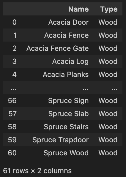
As you may have noticed, there are a lot of rows in this dataframe, and simply typing out “df” only shows the first several and last several rows. The “…” indicates that there are rows not visible.

You can see the total number of rows and columns at the bottom of the dataframe. In this case, we have 61 rows and 2 columns.
Head and Tail Link to heading
The function head shows us the first 5 rows by default.
df.head()
On the other hand, the function tail shows us the last 5 rows by default.
df.tail()
If we wanted to specify how many rows we wanted to see for either function, we just have to input the number of rows we want to see as an argument. For instance, let’s say that we want to see the first 10 rows of the dataframe:
df.head(10)
Or, if we want to see the last 15 rows:
df.tail(15)
iloc and loc Link to heading
We can also use the functions iloc and loc to extract information from dataframes. These functions return the information we want as a Series, which is a one-dimensional array of data.
The function iloc() uses numerical indices to identify the row and column of the data we want to call. Let’s see some examples.
# Print out the 1st row of the dataframe as a Series
# Remember that the indices starts from 0!
df.iloc[0]

# Print out the 37th row of the dataframe as a Series
df.loc[36]

# Print out the item in the 7th row and 1st column
df.iloc[6, 0]

# Print out the item in the 28th row and 2nd column
df.iloc[27, 1]
We can splice data by specifying the row and column indices we want. Splicing can return either a dataframe or a series.
# Return up to (not including) the 8th row of the dataframe -> returns a dataframe
df.iloc[:8]

# Return up to (not including) the 8th row in the first column -> returns a series
df.iloc[:8, 0]

# Return up to (not including) the 2nd column of the dataframe -> returns a dataframe
df.iloc[:, :1]

# Return all rows in the first column -> returns a series
df.iloc[:, 0]
We can also generate the same outcomes using loc(). The main difference is the loc uses the names of columns as an argument instead of their indices; it still uses indices for rows. Let’s see how we would write the code above using loc instead.
# Print out the 1st row of the dataframe as a Series
df.loc[0]

# Print out the 37th row of the dataframe as a Series
df.loc[36]

# Print out the item in the 7th row and 1st column
df.iloc[6, 'Name']

# Print out the item in the 28th row and 2nd column
We can also splice data with loc!
# Return up to (not including) the 8th row of the dataframe -> returns a dataframe
df.iloc[:8]

# Return up to (not including) the 8th row in the first column -> returns a series
df.iloc[:8, 'Name']

# Return up to (not including) the 2nd column of the dataframe -> returns a dataframe
df.loc[:, ['Name']]

# Return all rows in the first column -> returns a series
df.iloc[:, 'Name']
Ultimately, it comes down to personal preference for which one you want to use. Sometimes, it may be more intuitive to use indices, while other times, we may remember the column names better - there is no right or wrong choice!
Data Types Link to heading
Dataframes can contain many different data types such as strings, integers, floats or booleans. In short, strings are sequences of characters, like a word, phrase, or sentence; integers are numbers without decimal points; floats are numbers with decimal points; booleans are binary depictions of True or False values, usually depicted with 1 (True) and 0 (False).
To see what kind of data type our dataframe contains, we can use a function called type().
# Determine the type of data in the first column by extracting one object
type(df.iloc[0][0])
Running the above code should result in an output “str”, which indicates that the datatype we observed is a string! Since our dataframe does not contain any other datatypes, let’s practice using this function with simple data.
# The following code should print out "int" for "integer"
type(1)

# The following code should print out "float"
type(3.14)

# The following code should print out "bool" for "boolean"
type(False)
Columns Link to heading
Many times, we want to manipulate the columns in dataframe to organize our data. Some examples can involve adding columns of new, important information, or deleting columns to rid unnecessary data.
Creating Columns Link to heading
Let’s take a look at our data table again. That’s quite a lot of different types of wooden minecraft blocks! What if we want to look at the specific type of wood that each block is made of?
We can create a new column in the dataframe that extracts the our wanted data (the specific type of wood) from the first column. By observing our data, we notice that the material used for the minecraft block is the first word in our string. Since the datatype is a string, we can use .str functions to manipulate the data.
Since we want only the first word of each block name, we want to find someway to split the data first. We can use the function str.split(). The function takes in an argument, which specifies what we are splitting the string by (a space, a period, a letter).
# Try playing around with the function. What happens for each line?
df['Name'].str.split("a")
df['Name'].str.split("")
df['Name'].str.split(" ")
You may have observed that we want to split our string by a space, which is indicated by the last example above. This should split the data into something that looks like the image below.

How can we extract the first string? We can index into the first string with the following code:
df['Name'].str.split(" ").str[0]
Running the code above produces a series of our extracted data! Our final step is to add this series of data into a newly created column. To do that, we we can assign the code above into a newly created column, which we will call “Material”.
df['Material'] = df['Name'].str.split(" ").str[0]
df
When we run df now, we can see that there is a new column with all the data we just extracted. Since we have defined df to have this new column, it will continue to remain unless we write a code to remove it permanently.
Dropping Columns Link to heading
Let’s add a filler column to practice what we just learned first.
# Assign all rows a value of 1 in the column "Dummy".
df['Dummy'] = 1
Great! Now we have an example of a column that contains unnecessary data for our purpose. Looking at our dataframe, the column “Dummy” does not provide data that presents information we can draw conclusions from. So let’s get rid of it!
We can remove columns from our dataframe using the drop() function. Try the code below to see the dataframe generated.
df.drop(columns="Dummy")
The dataframe we just saw doesn’t show the “Dummy” column anymore right? But if we run df again…
df
… we still see the “Dummy” column. Why?
That is because when we dropped the column, we didn’t assign it back into the original dataframe variable, df. Just like how we had to assign a newly created column to df, we have to do the same if we want to permanently drop a column. Let’s code that out.
df = df.drop(columns="Dummy")
df
Now, when we run df, we see that the column “Dummy” has been completely removed from our dataframe.
Calling Columns Link to heading
Here are some techniques to return columns in a couple of different way.
Remember how we were able to use iloc and loc to call a column as a series? We can also perform the same task by writing:
# Returns a series
df['Name']
If we simply want to view a column as a dataframe instead of a series, we add another pair of brackets like so:
# Returns a dataframe
df[['Name']]
We can also call multiple columns in a dataframe:
# Returns a dataframe
df[['Name', 'Material']]
The rule above does not apply for series; remember, series are one-dimensional, and calling multiple columns would result in an error.
Grouping Data Link to heading
Sometimes, we want to be able to see the counts of data that belong to the same group. In this case, let’s analyze how many different types of blocks are in each material type.
We can use the function groupby() to “group” our data by material type. We would want to input the column name that we want to groupby as the argument, which in this case, would be “Material”. Let’s also assign this grouped dataframe into a new variable called “df_material”.
# We want to group the data by count
df_material = df_material.groupby('Material').count()
df_material
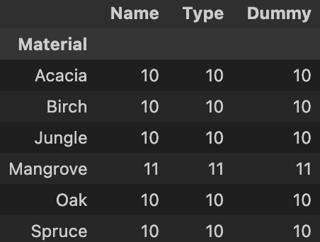
The code should produce a dataframe that looks like the one below.

As you can see, all the columns are now replaced by integers, which represent the count of each block type. Let’s rename one of our columns to “Count” (it doesn’t matter which one), and drop all the other ones. Feel free to follow my code exactly, or you can try it on your own!
df_material = df_material.rename(columns={"Name" : "Count"})
# axis=1 specifies that we are dropping columns
df_material = df_material.drop(['Type','Dummy'], axis=1)
df_material
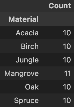
The dataframe printed should look like the one below.

Arithmetics Link to heading
Another way we can manipulate dataframe data is through mathematical procedures. In fact, it is very common to have to create new data (and often new columns) by using the raw data that was previously provided. Below describes
Simple Math Link to heading
We can also carry out mathematical procedures with the data in dataframes!
For instance, if we wanted to manipulate our counts in df_material, we can use the basic mathematical functions we know like below.
# Try out each of these lines separately to see what happens!
ddf_material['Count'] + 5

df_material['Count'] - 5

df_material['Count'] * 5

df_material['Count'] / 5
Let’s create a new column to store our calculated values.
df_material['Add 5'] = df_material['Count'] + 5
We can even carry out mathematical procedures among multiple columns in our dataframe! Call df_material to see the new columns.
df_material['Sum'] = df_material['Count'] + df_material['Add 5']
df_material
Inequalities Link to heading
What about inequalities and equalities? Checking inequalities and equalities result in dataframes that only contain the rows that hold true for the mathematical statements; this means that it is possible for an empty dataframe to be returned. Inequality and equality statements also work for strings
# We can check for lesser and greater than
df_material[df_material['Count'] < 10]

df_material[df_material['Count'] > 10]

# We can also check for "at most" and "at least"
df_material[df_material['Count'] <= 10]

df_material[df_material['Count'] >= 10]

# To check equality, we need to use two equal signs
df_material[df_material['Material'] == 'Acacia']

# The following code is checking for what is NOT equal to 'Mangrove'
df_material[df_material['Material'] != 'Mangrove']
Math Functions (And More) Link to heading
There are also some libraries that contain useful mathematical functions for us to use, such as pandas. The functions help us to quickly calculate data without having to write out every mathematical procedure out. Let’s take a look at some useful ones in the code below.
While calculating sums, mean, and median are relatively easy, they can be repetitive and tedious. Thankfully, pandas has functions that we can use.
# Calculate the sum
sum(df_material['Count'])

# Calculate the average
df_material['Count'].mean()

# Find the median
df_median['Count'].median()
We can also see how much unique data we have by using the function unique(). Let’s use our original dataframe df to see what are the unique types of materials for these blocks.
df['Material'].unique()
Notice how the materials are returned in an array? Calling unique tells us what the unique data are, not how many there are. To see how many there are, we can use the len() function.
len(df['Material'].unique())
This link provides an extensive list of useful functions (not just mathematical ones) that are commonly used.
Conclusion Link to heading
This concludes the first tutorial of working with dataframes. Hopefully, this has provided you with an insight into all the possibilities of working with a dataframe, as well as built your comfortability in exploring beyond what this tutorial has covered. Remember, the best way to familiarize yourself with working with dataframes (and coding in general) is to continuously use it. Be patient with yourself and try everything!